Ferromagnetic substances are those which gets strongly magnetised when placed in an external magnetic field. They have strong tendency to move from a region of weak magnetic field to strong magnetic field, i.e., they get strongly attracted to a magnet.
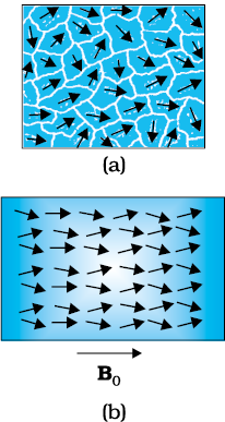
The individual atoms (or ions or molecules) in a ferromagnetic material possess a dipole moment as in a paramagnetic material. However, they interact with one another in such a way that they spontaneously align themselves in a common direction over a macroscopic volume called domain. The explanation of this cooperative effect requires quantum mechanics and is beyond the scope of this textbook. Each domain has a net magnetisation. Typical domain size is 1mm and the domain contains about 1011 atoms. In the first instant, the magnetisation varies randomly from domain to domain and there is no bulk magnetisation. This is shown in Fig. 5.13(a). When we apply an external magnetic field B0, the domains orient themselves in the direction of B0 and simultaneously the domain oriented in the direction of B0 grow in size. This existence of domains and their motion in B0 are not speculations. One may observe this under a microscope after sprinkling a liquid suspension of powdered ferromagnetic substance of samples. This motion of suspension can be observed. Figure 5.12(b) shows the situation when the domains have aligned and amalgamated to form a single ‘giant’ domain.
Thus, in a ferromagnetic material the field lines are highly concentrated. In non-uniform magnetic field, the sample tends to move towards the region of high field. We may wonder as to what happens when the external field is removed. In some ferromagnetic materials the magnetisation persists. Such materials are called hard magnetic materials or hard ferromagnets. Alnico, an alloy of iron, aluminium, nickel, cobalt and copper, is one such material. The naturally occurring lodestone is another. Such materials form permanent magnets to be used among other things as a compass needle. On the other hand, there is a class of ferromagnetic materials in which the magnetisation disappears on removal of the external field. Soft iron is one such material. Appropriately enough, such materials are called soft ferromagnetic materials. There are a number of elements, which are ferromagnetic: iron, cobalt, nickel, gadolinium, etc. The relative magnetic permeability is >1000!
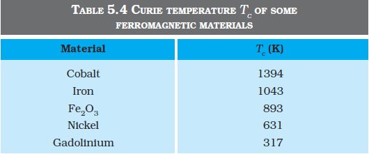
The ferromagnetic property depends on temperature. At high enough temperature, a ferromagnet becomes a paramagnet. The domain structure disintegrates with temperature. This disappearance of magnetisation with temperature is gradual. It is a phase transition reminding us of the melting of a solid crystal. The temperature of transition from ferromagnetic to paramagnetism is called the Curie temperature Tc. Table 5.4 lists the Curie temperature of certain ferromagnets. The susceptibility above the Curie temperature, i.e., in the paramagnetic phase is described by,
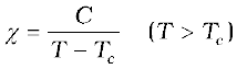 (5.21)
Example 5.11 A domain in ferromagnetic iron is in the form of a cube of side length 1µm. Estimate the number of iron atoms in the domain and the maximum possible dipole moment and magnetisation of the domain. The molecular mass of iron is 55 g/mole and its density is 7.9 g/cm3. Assume that each iron atom has a dipole moment of 9.27×10⁻²⁴ A m2.
Solution The volume of the cubic domain is
V = (10–6 m)3 = 10–18 m3 = 10–12 cm3
Its mass is volume × density = 7.9 g cm–3 × 10–12 cm3= 7.9 × 10⁻¹² g
It is given that Avagadro number (6.023 × 10²³) of iron atoms have a mass of 55 g. Hence, the number of atoms in the domain is
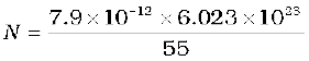
The maximum possible dipole moment mmax is achieved for the (unrealistic) case when all the atomic moments are perfectly aligned. Thus,
mmax = (8.65 × 1010) × (9.27 × 10–24)
= 8.0 × 10⁻¹³ A m2
The consequent magnetisation is
Mmax = mmax/Domain volume
= 8.0 × 10⁻¹³ A m2/10–18 m3
= 8.0 × 10⁵ Am–1
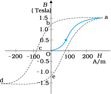
The relation between B and H in ferromagnetic materials is complex. It is often not linear and it depends on the magnetic history of the sample. Figure 5.14 depicts the behaviour of the material as we take it through one cycle of magnetisation. Let the material be unmagnetised initially. We place it in a solenoid and increase the current through the solenoid. The magnetic field B in the material rises and saturates as depicted in the curve Oa. This behaviour represents the alignment and merger of domains until no further enhancement is possible. It is pointless to increase the current (and hence the magnetic intensity H) beyond this. Next, we decrease H and reduce it to zero. At H = 0, B ≠ 0. This is represented by the curve ab. The value of B at H = 0 is called retentivity or remanence. In Fig. 5.14, BR ~ 1.2 T, where the subscript R denotes retentivity. The domains are not completely randomised even though the external driving field has been removed. Next, the current in the solenoid is reversed and slowly increased. Certain domains are flipped until the net field inside stands nullified. This is represented by the curve bc. The value of H at c is called coercivity. In Fig. 5.14 Hc ~ –90 A m–1. As the reversed current is increased in magnitude, we once again obtain saturation. The curve cd depicts this. The saturated magnetic field Bs ~ 1.5 T. Next, the current is reduced (curve de) and reversed (curve ea). The cycle repeats itself. Note that the curve Oa does not retrace itself as H is reduced. For a given value of H, B is not unique but depends on previous history of the sample. This phenomenon is called hysterisis. The word hysterisis means lagging behind (and not ‘history’).
Hysterisis in magnetic materials:
http://hyperphysics.phy-astr.gsu.edu/hbase/Solids/hyst.html
© 2026 GoodEd Technologies Pvt. Ltd.

